Continuing from yesterday, the process of constructing the neural network is relatively simple once the activation function is understood. All that needs to be done is stack up layers with activation functions in between. We can have as many as we like, with as many neurons as we like in each hidden layer. Sometimes they bloat up like this for huge problems:

There’s one last layer we need at the end though. The output layer will narrow the data down to certain classes because in this case we’ll be making a neural network known as a classifier. A classifier takes input data and tries to predict which class the data falls into based on previous features that have been trained into the network. For example, you taught one of these to recognize cats, it would have two output neurons, ‘Cat’ and ‘Not Cat.’ You could add in ‘Dog,’ and change ‘Not Cat,’ to ‘Unknown.’ Or add as many output classes as you wanted. Go nuts.

You might be wondering how this classification is actually determined though. Yesterday we saw that the ultimate result of a layer of neurons is just a big bunch of numbers pumped into the rectified linear activation function. How do these activation numbers predict what something is.

Output neurons will activate according to a function whose inputs are of all the previous weights, biases, and activation functions. If you want this to look a little more severe …

output = w_{i *} f_L (w_i * f_L-1 (w_i * f_L-2 (w_i * x_i)))

where x_i are the initial inputs to a network with two hidden layers. Subscript L is the last layer. L-1 is the previous layer, and so on. If you’re wondering why I didn’t include biases, we’ll get to that later. Just know for know we don’t really need to see them in there to understand what’s going on.

The output of the network is a function of functions. Each output neuron will just spit out a number like all the rest if we do nothing different. What we need is to change our function in between that last hidden layer and the output layer.

I finally found a diagram that includes the activation functions by the way.

See the red boxes? Shout out to Alexander Eul there for making this.

There’s a problem with our network compared to the diagram. That last output in the diagram is a probability value. If we continue to use rectified linear activation functions the whole way through, we’ll never see any probabilities.

We could just ignore this though.

What if we take the last output of all the neurons (using rectified linear the whole way through), and say “hey, this neuron’s output is greater than all the rest. Let’s just use that our classification.”

As you can see in the diagram, it does basically the same thing. The ultimate result is a one or a zero for each category, so why bother with calculating a probability beforehand?

The answer has to do with training. It would be useful to know not just when the network is wrong, but how wrong it actually is, also known as loss.

Imagine someone was teaching you to write the perfect essay. You write essays, submit them to a grader, and have them returned. If you want to learn, you’ll need to improve on your mistakes. But what if instead of marking your mistakes individually, the grader simply told you the essay as a whole was either good or bad? 1 or 0. Every time you submit a good essay you have no idea why it was good, just that it was. Every time you submit a bad essay you have no idea why it was bad either. That would be pretty difficult to learn from, right? What if all the things you included in one of the bad essays were actually good features except for one failure that the grader particularly hated? You would consider changing everything about the essay even if it was only one issue that made it ‘bad.’ It would be confusing and easy to overcompensate to say the least.

That’s what happens when our classifier only puts out a 1 or 0 for each class. That data is extremely hard to train it with. Instead we want a percentage that represents how confident the network is that any given inputs fall into a certain class. With that we can go back and tell the network “this was 90% accurate, please only try to improve by 10%.”

So then, it should be easy. Just take each output from the final layer, and divide it by the sum of all the outputs of the final layer. That will give us the percent of the total output that each neuron in the output layer has.

Only one problem. What if our final outputs look like this?

Neuron 0 -> 2
Neuron 1 -> -1
Neuron 3 -> -1

If we try to get a probability here, we end up dividing by 0.

Neuron 0 / (Neuron 0 + Neuron 1 + Neuron 2)

2 / (2 – 1 – 1)

2 / 0

Uh oh. But that’s ok. Let’s just remove the negative values. They’re just negatives, right?

Neuron 0 -> 2
Neuron 1 -> 0
Neuron 3 -> 0

2 / (2 + 0 + 0) = 1

But wait, now the final output indicates that the network was 100% confident that the class represented by Neuron 0 was the right one. That’s not entirely true, is it? The other outputs may have been negative, but they still had non-zero values. Clearly there was more going on in the network that we failed to capture. We can’t use this data to make any improvement because the network already thinks that it’s perfect.

We need to remove the negative values without removing the information they represent.

Introducing, the exponential function.

This function is great because no matter how negative the input is, the output of the function will always be a positive number. We can use this to eliminate negative values without completely destroying their useful information.

If you’re wondering what e is, that’s Euler’s number. It’s special in that the derivative of e^x = e^x Don’t worry about that right now though.

e^-1 evaluates to 1 / e by the rules of exponents. e^-2 would evaluate to 1 / e² , e^-3 to 1 / e³ and so on.

This is why the exponential function never becomes negative, but the values do get smaller and smaller because it divides by a larger and larger number.

Let’s calculate that probability again.

Neuron 0 -> 2 -> e²
Neuron 1 -> -1 -> e^-1
Neuron 3 -> -1 -> e^-1

e² / (e² + e^-1 + e^-1) = ~0.91

Or about 91% confidence that our inputs fall into class 0.

Doing all those steps together is called the softmax function. Here’s a more thorough representation:

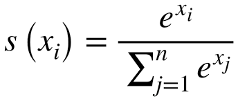
Where n is the total number of outputs from the output layer, and i represents the individual output that you’re trying to calculate a percentage for. The E thing is called sigma, and is just a fancy way to write “do a sum of all the output neurons.”

Now that we have this percentage we can calculate loss, a numeric value representing the ‘wrongness’ of the whole network. Then we can use that value to backpropagate corrections to the weights.

I’ll have to leave that for tomorrow though. I thought I’d be able to wrap this up today but every step is more complicated to write out than it was in my mind. This was mostly just to cement all this information into my brain anyway, so I’m happy to take it a little slow. Tomorrow I’ll definitely be finished though, because my knowledge of the topic will run out!

I’ll have my review for ‘The Forest for the Trees’ ready on Monday if you’ve been looking forward to that and wondering what on Earth all this mathematical crap is doing here. I’ll go back to regularly scheduled programming … eventually.

Thank you for reading,

Benjamin Hawley