Today will be the last post explore the neural network established over the past week. We’re to the final stage of initializing the network. It’s output some data and we used the softmax function to attain a set of probabilities. Now there’s just the question of what to do with them. What I’ll be covering today is called backpropagation, taking the loss and using it to refine the weights and biases of the network. It’s very complex, and can be done multiple ways, so this post will be a high level overview of how it actually works.

I should mention some more vocabulary before beginning. The set of probabilities our model outputs is called a probability vector. A vector is just a one dimensional set of numbers, like this:

[0.3, 0.4, 0.3]

For a probability vector they should all add up to one, since the combined probability of every output is the essentially the probability that the output exists, which we know is 100%.

If you graph a vector it’ll look like an arrow. This is important for later, and I encourage you to play around with this calculator to understand what a vector is visually.

We can take our probability vector and calculate a loss using another function called categorical cross-entropy. This is a loss function specifically for calculating loss across three or more categories. There is a binary function that works similarly, but I’ll be focusing on this one.

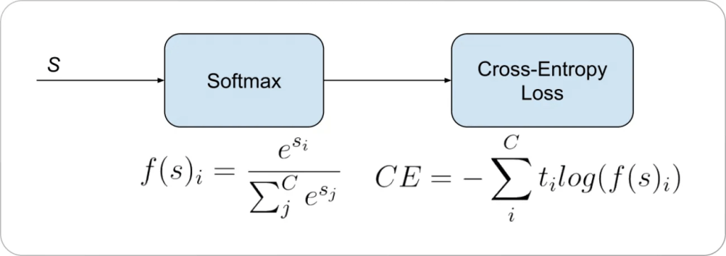
There’s our softmax function on the left, whose outputs we can put straight into the cross-entropy loss formula. We simply multiply each category’s expected value by the negative log of the actual output and add them all together. Since we assume any given input can only fall into one category (this is not always the case, but is much simpler), our expected output will always look something like this:

[1,0,0] or [0,1,0] or [0,0,1]

Effectively this means that the cross-entropy function will multiply any incorrect output values by zero, then score the predicted category against the actual category.

The value of loss for any given output will increase as the output of the softmax function decreases. This is important to wrap your head around, so here’s a handy graph:

The loss of the system actually approaches infinity if you happen to have a 0 output for any particular category. This can be solved by capping loss at a very high value, so don’t worry about it. The important part is that the further our prediction is from the true category the input data falls into, the greater the loss will become.

Unfortunately for us, these models do not come out of the box ready to predict anything with any sort of accuracy. At first, all the weights will be small randomized values. Every output to any input will therefore predict that there is an equal likelyhood of the input data falling into any given category. In other words, the network has no idea what it’s looking at, so it just says “eh, could be anything.”

[0.333, 0.333, 0.333]

On average, we’d expect every single output to look like the above no matter how many times we ran an input through the network. This is where loss really comes into play.

Remember how I said that this network is giant function made up of other sub-functions? The same is true for the loss function. All it does is further manipulate the output of the network. The loss function can be represented as follows.

Loss = C(y, f_L(w_{L *} f_L-1 (w_L-1 * f_L-2 (w_L-2 * f₁ (w₁ * x)))))

This is a slightly altered version of what I had yesterday, where the loss is a function that takes inputs y, the true value of the category, and the entire output of the rest of the network.

What we want is to minimize this function. It represents everything that is wrong with our network. We already included a method of changing this output by updating the weights and biases accordingly. The biases are not as crucial as the weights, and you’ll see why in a moment.

What we could do is just randomly adjust weights and always save the best outcome as the model. It would improve as we did this over and over again, recalculating loss each time and checking it against the loss of the previous iteration. This is not very intelligent though, and it doesn’t work well in most situations. It’s also painfully slow if you do want to achieve a certain level of accuracy. It’s random, so there’s no guarantee you’ll ever get there either.

What’s smarter is to use calculus. Using calculus, we could find the slope of this giant function, or in this case, the gradient, which is a vector (recall the arrows) of all the partial derivatives of the function. This giant function representing loss actually takes multiple inputs all once. That means for each layer we’ll have to take the derivative with respect to each individual input.

If you don’t know calculus, you may not understand what that means. Essentially, a function’s output is related to the input in some way. This seems trivial, but if you ask the question, “how fast is a function’s output changing as its input changes?” you will go down the same line of questioning that brought Isaac Newton to discover calculus.

A basic derivative is just the slope of a line. y = x has a slope of 1, because for each increment in x, y increases by 1. y = 2x has a slope of 2, and a derivative of 2.

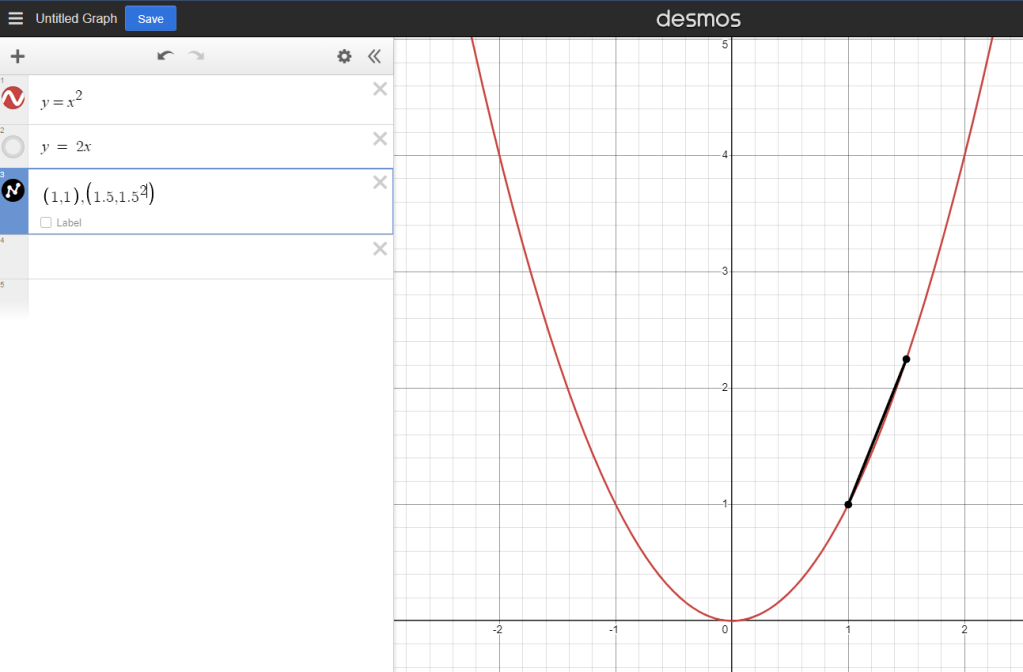
This gets more complex with larger functions, where the slope of the line actually changes too. On a straight line the slope never changes, but what about something like this?

Here’s it’s much harder to say how the line is changing because if you try to do a rise/run or a change in y / change in x calculation, you actually just calculate a straight line.

See how the black line overestimates the red line? This rate of change is not accurate. It becomes more accurate as the change in our x value decreases though.

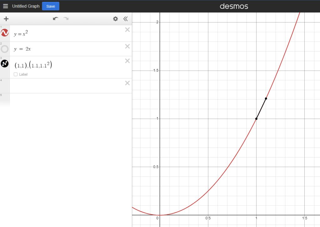
Now it’s almost perfect. But what if we reduce it even further? What if the difference between the X values was actually 0? Well you can’t divide by zero, but we know that at any given point the function is still changing, otherwise it wouldn’t grow at all.

Turns out there are a handy set of rules to figure this out.

Deriving them is harder, but you can just take Isaac Newton’s word for it frankly.

But our function takes multiple inputs …

Loss = C(y, f_L(w_{L *} f_L-1 (w_L-1 * f_L-2 (w_L-2 * f₁ (w₁ * x)))))

A ton of them in fact. Well, that’s fine, says Newton. You can just find the derivative with respect to one input at a time. This is called a partial derivative, and I’m not sure I have the stamina to explain those too. I encourage you to read about them on your own.

Taken all together, partial derivatives form a gradient. You can think of this as an arrow that points in the direction the function is growing or shrinking. It’s easier to see visually if you don’t fully understand derivatives. Gradients make for very pretty vector fields, where each set of inputs to the partial derivatives generates an arrow pointing in the direction the function is changing in. Here’s what they look like:

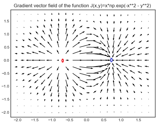
You can use these to graph magnetic fields, which is why that one there looks so familiar. Here’s a similar one in three dimensions.

At any point on this graph, the gradient allows us to calculate how the function is changing as our inputs change. At points where the vector field touches the bottom, the function is not changing at all, and has reached a minimum … and what were we trying to do again? Oh yeah, find a minimum for our loss function! Perfect.

We would very much like to find ourselves in one of those pits … ok that may have come out wrong, but you see what I mean. We can generate a gradient for each layer of neurons and use it to push our loss closer and closer to 0. This is done by segmenting out the gradient using a method called stochastic gradient descent, but this topic would probably cover a whole other post.

Backpropagation is the key to training a neural network, and the last step I’ll be covering in this series. Frankly the derivation of those gradients is scary. Here is how you can take the derivative for categorical cross-entropy loss. As you can see it simplifies down to something really nice, just the true expected output divided by the predicted output times -1, which we can code into the computer to calculate the gradient. Getting there is harder however.

This is just one step too, you need to do this for every single different function we used along the way! If you wanted to implement a custom loss function you’d have to do it all by yourself too, because more than likely nobody else has taken the time to do it for you. I’m not there yet, so I’ll stick to copying the derivatives out of this great book I bought on the subject that you can find right here. It’s not cheating, it’s efficient, ok?

Ok maybe it still feels like cheating. Whatever, it gets the job done, and I think I know what it’s doing … most of the time.

So that’s the gist of how a neural network functions. Pretty complicated, but if you can remember:

1. Layer output = inputs * weights + biases
2. Rectified linear activation function = max(layer output, 0)
3. Predicted category = exponential function of the final neuron output / the sum of exponential of all the final outputs
4. Backpropagation is just finding bunch of tiny arrows and following them into a deep, dark hole

Then you probably understand more than 99% of people. At least, for supervised networks. There are other kinds of networks that do not backpropagate in the same way … that’s a topic for a more informed me to write about though.

Thank you for reading,

Benjamin Hawley