Yesterday I started on a rather convoluted topic, but hopefully if you wrapped your head around what a layer does to the inputs it receives, then today’s post should be easier to understand. Here was the output of the layer from yesterday’s example.

	N1	N2	N3	N4	N5
Output	0.62	0.455	0.975	0.18	0.125

What we’d like to do is pass these values to a new layer. Recall that each layer has neurons with weights and biases, like knobs on a large machine. Passing these values to a new layer would allow even finer control over the effect the network has on the inputs. Deciding how many layers is a whole other topic, but for now we can just assume that two layers will be better than one. In fact, two layers between the first input and the final output is pretty much required for reasons I’ll try to explain right now.

We can’t simply pass these inputs along to a new layer, or to the final output layer. As stated yesterday, the function these neurons apply to their inputs is this:

output = inputs x weights + bias

This is identical to the equation of a line.

y = mx + b

Where the weights determine the slope of the output line (m), and the bias determines the intercept of the line (b). Currently, all our neural network can do is take inputs and turn them into lines. No matter how many layers we stack up on top of each other, the output will always look like a line because all we are doing is multiplying previous inputs by a new slope. Most data in the real world does not have a perfectly linear relationship.

The whole thing is useless! That is, if we leave it as is. To solve this, the linearity of the system must be broken. There needs to be a way to introduce curves or kinks into these lines. What if we could have a neuron or a couple of neurons only define one section of a line? Then we could make a curve that’s just a bunch of tiny line segments. We might then say that some neurons are active for certain inputs. I.E any given neuron can only contribute to the line when we want them to. This is exactly what an activation function achieves.

An activation function sits between layers of neurons and decides which neurons will get to play their part. It’s part of the picture that’s missing from diagrams like these:

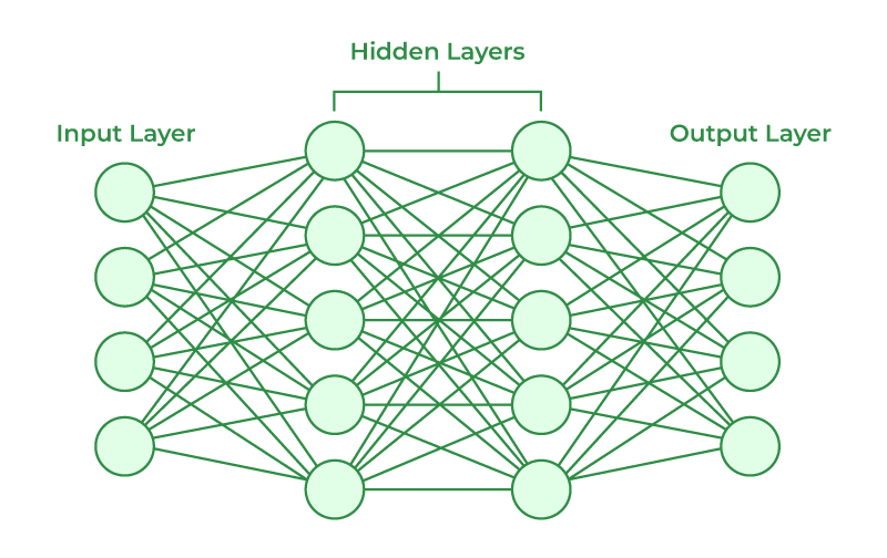
In fact I couldn’t find a single diagram that indicates the existence of an activation function between neurons. They’re such an integral part of these networks it’s kinda hard to believe nobody includes them in the diagram.

Anyway here’s a visual for how they work.

First we just start with a line. If we take the input and our entire neural network was active at the same time, we’d get something like this:

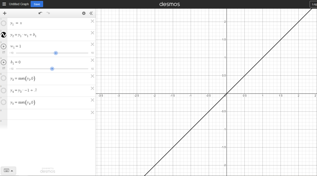
Those sliders, w1 and b1 determine the slope and position of the line. Those could be just one weight, or they could be every weight and bias added together. If every neuron is always active, all the neurons’ weights and biases will end up multiplied or added to the final output. That’s why we’ll always get a line (or at least, a representation of a linear relationship) without any activation function.

Changing weight:

Changing bias:

Today we’ll be looking at the rectified linear or ReLI activation function. All it does is cut a line off where it’s output is not greater than 0. This is enough to break linearity and allow us to make some more interesting shapes.

This next line is what happens when the activation function is applied it’s active where the original input is between 0 and infinity.

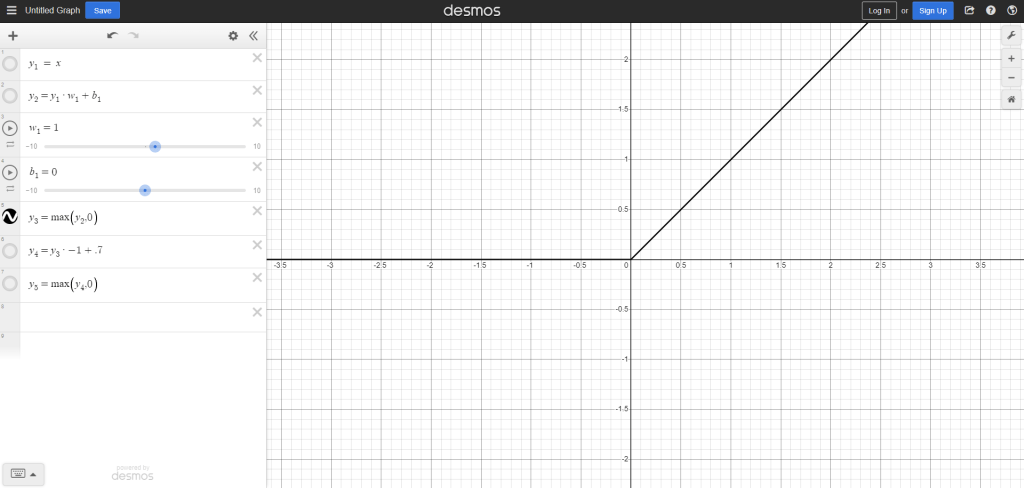
Notice these aren’t completely new lines, I’m taking the output of the previous function and doing new operations to it, just like the neural network will.

Now what if I want a line that’s active only over a constrained area like we talked about before? I need to do a few operations. First I’ll pass the output of the activation function to a new neuron, and use the weight and bias to set some limits.

Then I have to pass this to another activation function.

And there you go, the output is no longer just a single line. I can even reverse this again by applying one last weight to it as it’s accepted by the output neuron to get this.

This is about as simple as I can possibly get. This neural ‘network’ would just be four neurons. Input neuron that receives X values, two hidden neurons, and a final output neuron that gives us the Y values as displayed in the calculator. Stack several of these neuron pairs together and you can make a curve, as demonstrated in this video with much more depth:

Something to keep in mind is that these outputs are lines because I’ve used two neurons, or as he does in the video, neuron pairs. For a dense layer as we explored yesterday, the output could be reduced to lines at the very end if that were your prerogative, but the actual output of each individual layer is impossible to visualize. Those matrix multiplications we were doing yesterday can get into the hundreds of dimensions. This was a simplified example for the sake of figuring out what the heck is going on in there.

That’s about it for the rectified linear activation function. Tomorrow I’ll finish this neural network series up with one more post, and then I’ll move on to my usual book review and literary content. I wanted to give more technical writing a try and found out it’s pretty hard. I’ll have some good material to look back on and learn from, and maybe in the future I’ll give some other technical concept a try.

Thank you for reading,

Benjamin Hawley