I took a break from writing over the weekend to explore a little in a totally different field. I find it’s good to broaden my horizons as much as I can to find new sources for my writing. In this case, I also just really wanted to know how machine learning algorithms actually function. You see them all over the news these days, from complex models like ChatGPT and the perceptrons behind self-driving cars, to simple sentiment analyzers that allow huge corporations to figure out how everyone who has ever posted about them feels about the company. Everyone seems to believe these models are the future, for better or worse. If they’re right, then I must ask, how will this future actually function at a fundamental level? That’s what I wanted to figure out, so I built one.

First I need to constrain what I’m talking about though. Machine learning encompasses a huge field. What I was interested in is called deep learning, where neural networks are used to extract and classify input data. What I find most interesting about neural networks is that they’re specifically designed to mimic the decision making capability of organic brains. Our eyes send us images, and based on that data, we can tell we’re looking at a cat, or a dog, or even if we’re looking at something we’ve never seen before. We can find patterns in sequences of numbers, search for meaning in text, and identify each other based on the sound of our voices. These are all problems encompassed by deep learning that can be solved using neural networks.

Not all machine learning is deep learning. Deep learning specifically refers the use of a neural network to extract features and classify data based on those features. Machine learning applications can classify data without the use of such a complex algorithm as a neural network and are actually much better in many scenarios. There are some other major differences you can read more about at here at turing.com. Just wanted to make that clear before we move on.

Here’s the gist of a neural network. You may have seen something similar before:

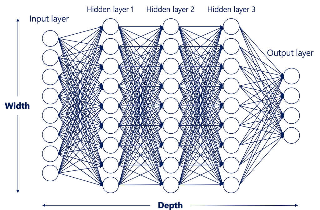
Inputs come in, stuff happens, outputs come out. Simple. And actually, when you dig into the individual steps, they are simpler than you might expect. It’s by combining a large number of simple steps that these algorithms achieve their complexity. Let’s start with the neuron, the circles you see up there. What are they really? They actually only hold a couple pieces of information:

Neuron
– Weights
– Bias

That’s it. Each of those circles has nothing but. And in fact, they don’t even really exist as you might think of them. There is no object called a neuron in any neural network as far as I’m aware. That’s because there’s a better way to represent them. Putting them into layers of neurons is much easier than creating a hefty container for each and every neuron. It will become obvious why this is the case as you keep reading.

Each layer looks more like this when you’re actually working with them:

Weights:
[

[-0.2, 0.01, 0.1, -0.01, 0.04],
[ 0.01, -0.02, 0.1, -0.02, -0.01],
[ 0.1, 0.17, 0.25, 0.06, 0.06],
[ 0.2, -0.01, -0.03, 0.02, -0.03]

]

Biases:
[[0, 0, 0, 0, 0]]

Maybe you’re thinking, ew, numbers. It’s not as bad as it looks. Each bracketed set of numbers [ ] is called an array. Both of these are arrays of arrays, or two dimensional arrays.

In the weights array, the number of rows indicates how many inputs the layer will receive. In this case four rows, so four inputs. Those four inputs could come from a previous layer, but for this particular example, each sample of our input data is made up of four numbers, like this:

Inputs:
[

[1, 2, 3, 2.5]

]

That’s a single sample. Later we might look at multiple samples, but for now, it’ll be just the one.

But back to the weights array. The number of columns indicates the number of neurons in the layer, in this case five.

1 2 3 4 5
[-0.2, 0.01, 0.1, -0.01, 0.04],
[ 0.01, -0.02, 0.1, -0.02, -0.01],
[ 0.1, 0.17, 0.25, 0.06, 0.06],
[ 0.2, -0.01, -0.03, 0.02, -0.03]

Each number in a column represents the weight of the input to the neuron that the column represents. You could think of this weight as how much credence the neuron will give each input. A big weight means that particular input will have a big impact on the output of the neuron. A small weight will reduce the impact of the input to the neuron. These are adjusted later to tune the network during training.

Next up, the biases. Each neuron has one bias. There are five columns in the weights array, so there should be five columns in the biases array. You might be wondering, why not one bias per input, per neuron like we have with weights? This is to give the network the ability to adjust different aspects of the system later on. Different kinds of knobs on the machine, so to speak.

How are these actually used by each neuron? It’s a simple formula:

output = sum (weights x inputs) + bias

This layer has five neurons. Each neuron takes four inputs and has one weight associated with each input. It multiplies each input by each weight, then adds them all together, and adds the neuron’s bias on top of that. 20 multiplications, and then it sums them up. A larger network might look like this.

Each line is a weight associated with the previous neuron’s output, which becomes the next neuron’s input. The biases aren’t listed, but frankly they aren’t as important as the weights anyway. Each neuron has only one output, but that output is piped to each neuron in the next layer.

You might still be wondering, why put them in layers? Because a nice mathematician named Lagrange invented a something called the dot product way back in 1773. Today, we use the dot product to trick rocks into thinking for us. Crazy.

Anyway the dot product is at the heart of matrix multiplication. A matrix is essentially just like an array, at least for our purposes today. Here is an image I stole from Medium.

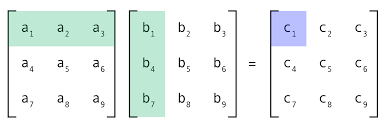
It’s not too complicated, but it does stretch your brain a little. Multiply each element in the row by each element in the column, then add them all together to get one number. Do this for every combination of rows and columns, and you’ll end up with a new matrix at the end.

Using this technique, we can do all the multiplication and addition we need all at once rather than going one neuron at a time. Hence putting the neurons into ‘layers’ which are actually just arrays, which act exactly like a matrix in this case … Getting kinda convoluted here, but if you’re still following, here’s a cookie.

Here’s our inputs again, tidyed up some to look more like a matrix.

[1, 2, 3, 2.5]

And our weights

[-0.2, 0.01, 0.1, -0.01, 0.04]
[ 0.01, -0.02, 0.1, -0.02, -0.01]
[ 0.1, 0.17, 0.25, 0.06, 0.06]
[ 0.2, -0.01, -0.03, 0.02, -0.03]

First multiply each of these, then add the results together.

[1, 2, 3, 2.5]

[-0.2, 0.01, 0.1, -0.01, 0.04]
[ 0.01, -0.02, 0.1, -0.02, -0.01]
[ 0.1, 0.17, 0.25, 0.06, 0.06]
[ 0.2, -0.01, -0.03, 0.02, -0.03]

Then the next column.

[1, 2, 3, 2.5]

[-0.2, 0.01, 0.1, -0.01, 0.04]
[ 0.01, –0.02, 0.1, -0.02, -0.01]
[ 0.1, 0.17, 0.25, 0.06, 0.06]
[ 0.2, –0.01, -0.03, 0.02, -0.03]

Then the next …

[1, 2, 3, 2.5]

[-0.2, 0.01, 0.1, -0.01, 0.04]
[ 0.01, -0.02, 0.1, -0.02, -0.01]
[ 0.1, 0.17, 0.25, 0.06, 0.06]
[ 0.2, -0.01, –0.03, 0.02, -0.03]

And so on until you get this, one number per column because remember each column represents a neuron.

	N1	N2	N3	N4	N5
Output	0.62	0.455	0.975	0.18	0.125

Then add all the biases of each neuron to each output, which were all 0 if you remember, so we don’t need to do anything more.

This is the output of the layer.

As these are just random numbers, the output is completely meaningless. It was just to help understand what the layer is actually doing.

Tomorrow I’ll go over what the network actually does with this layer’s output. After writing all this out, I realized how much background knowledge it really takes to grasp this. Without prior understanding of matrix multiplication, it can take some time to wrap your head around it. I didn’t expect the post to go on so long honestly. Sorry about that. If you’re still confused, here’s a Khan Academy lesson on matrix multiplication that should help.

Just remember: Weights times inputs plus the bias! If you can wrap your head around weights times inputs, then you’ll have everything you need for tomorrow’s post.

Thank you for reading,

Benjamin Hawley